Exact GP Regression Tutorial

Introduction

In this notebook, we use DMGP to train a simplest regression model. We’ll be modeling the function \begin{align} &y = \sin(2\pi x) + \epsilon, \\ &\epsilon \sim \mathcal{N}(0,0.04). \end{align} with 100 trianing examples, and testing on 50 test examples.

Note: this notebook is not necessarily intended to teach the mathematical background of Gaussian processes, but rather how to train a simple one and make predictions in DMGP. For a mathematical treatment, please see the reference “A sparse expansion for deep Gaussian processes”: https://arxiv.org/abs/2112.05888

import math
import numpy as np
import torch
import torch.nn as nn
import torch.nn.functional as F
from dmgp.models import DMGP
from dmgp.layers.activation import TMK, AMK
from dmgp.layers.linear import LinearFlipout

Set up training data

In the next cell, we set up the training data for this example. We’ll be using 100 regularly spaced points on [0,1] which we evaluate the function on and add Gaussian noise to get the training labels.

# Training data is 100 points in [0,1] inclusive regularly spaced
train_x = torch.linspace(0, 1, 100)
train_y = torch.sin(train_x * (2 * math.pi)) + torch.randn(train_x.size()) * 0.2
x_tensor = train_x.view(-1, 1)
y_tensor = train_y.view(-1, 1)

Setting up the model

The next cell demonstrates the most critical features of a user-defined DGP model in DMGP. Basically, there are two ways to define a customized DGP model: use dmgp.models.DMGP or construct your model from scratch using dmgp.layers.

If we define the model using dmgp.models.DMGP, you need to construct the following DMGP objects: 1. Input and output dimension (input_dim, output_dim) - For regression output_dim=1. 2. Number of hidden layers (num_layers) - Usually we use 2 hidden layers. 3. Level of inducing (num_inducing) - This sets the level of inducing points we use for GP inference. 4. Dimension of hidden layers (hidden_dim) - This sets the width of hidden layers. 5. A kernel (kernel) - This defines the prior covariance of the GP. (In DMGP, DMGP.kernels.laplace_kernel.LaplaceProductKernel is a good choice to start). 6. A layer type (layer_type) - This defines the linear Bayesian layer we use for learnable GP weights. (DMGP.layers.linear.LinearFlipout is used by default).

from dmgp.utils.sparse_design.design_class import HyperbolicCrossDesign
from dmgp.kernels.laplace_kernel import LaplaceProductKernel

# Define the model using DMGP
dmgp_model = DMGP(in_features=1,
                  out_features=1,
                  num_layers=2,
                  hidden_dim=8,
                  num_inducing=3,
                  input_lb=0,
                  input_ub=1,
                  kernel=LaplaceProductKernel(1.),
                  design_class=HyperbolicCrossDesign,
                  linear_layer=LinearFlipout,
                  option='additive')

If we define the customized model from scratch, the following is an example which consists of two GP layers, each with level-8 and level-5 sparse grid design, respectively.

# Define a DMGP model from scratch
class DMGP_regression(nn.Module):
    def __init__(self, input_dim, output_dim, design_class, kernel):
        super(DMGP_regression, self).__init__()

        # 1st layer of DGP: input:[n, input_dim] size tensor, output:[n, 1] size tensor
        self.mk1 = AMK(
            in_features=input_dim,
            n_level=5,
            input_lb=0,
            input_ub=1,
            kernel=kernel,
            design_class=design_class,
        )
        self.fc1 = LinearFlipout(self.mk1.out_features, 1)

        # 2nd layer of DGP: input:[n, 1] size tensor, output:[n, output_dim] size tensor
        self.mk2 = AMK(
            in_features=1,
            n_level=5,
            input_lb=0,
            input_ub=1,
            kernel=kernel,
            design_class=design_class,
        )
        self.fc2 = LinearFlipout(in_features=self.mk2.out_features, out_features=output_dim)

    def forward(self, x, return_kl=True):
        kl_sum = 0
        x = self.mk1(x)
        x, kl = self.fc1(x)
        kl_sum += kl
        x = self.mk2(x)
        x, kl = self.fc2(x)
        kl_sum += kl
        if return_kl:
            return x, kl_sum
        else:
            return x

model = DMGP_regression(
    input_dim=1,
    output_dim=1,
    design_class=HyperbolicCrossDesign,
    kernel=LaplaceProductKernel(1.),
)

Training the model

In the next cell, we handle using variational inference (VI) to train the parameters of the DMGP.

criterion = nn.MSELoss()
optimizer = torch.optim.Adam(model.parameters(), lr=0.01)

# Training loop
epochs = 1000
for epoch in range(epochs):
    model.train()
    optimizer.zero_grad()
    output, kl = model(x_tensor)
    loss = criterion(output, y_tensor) + kl/len(train_x)
    loss.backward()
    optimizer.step()

    if epoch % 100 == 0:
        print(f'Epoch [{epoch}/{epochs}], Loss: {loss.item()}')

Epoch [0/1000], Loss: 0.6518664360046387
Epoch [100/1000], Loss: 0.22241495549678802
Epoch [200/1000], Loss: 0.14881879091262817
Epoch [300/1000], Loss: 0.13053223490715027
Epoch [400/1000], Loss: 0.1292726993560791
Epoch [500/1000], Loss: 0.1213754415512085
Epoch [600/1000], Loss: 0.11744579672813416
Epoch [700/1000], Loss: 0.1487128734588623
Epoch [800/1000], Loss: 0.13028332591056824
Epoch [900/1000], Loss: 0.12365931272506714

Making predictions with the model

In the next cell, we make predictions with the model. To do this, we simply put the model in eval mode, and call both modules on the test data.

# Test points are regularly spaced along [0,1]
test_x = torch.linspace(0, 1, 50)
test_y = torch.sin(test_x * (2 * math.pi))
test_x = test_x.view(-1, 1)
test_y = test_y.view(-1, 1)

# Make predictions by feeding test dat through DMGP model
test_loss = []
with torch.no_grad():
    predicts = []
    for mc_run in range(20):
        model.eval()
        output = model.forward(test_x, return_kl=False)
        loss = F.mse_loss(output, test_y).cpu().data.numpy()
        test_loss.append(loss)
        predicts.append(output.cpu().data.numpy())

    pred_mean = np.mean(predicts, axis=0)
    pred_std = np.std(predicts, axis=0)

print('test loss: ', np.mean(test_loss))

test loss:  0.06484331

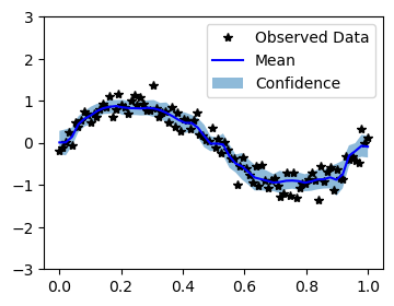
Plot the model fit

In the next cell, we plot the mean and confidence region of the DMGP prediction.

from matplotlib import pyplot as plt
from scipy import stats

# Confidence level
confidence_level = 0.95
z = stats.norm.ppf(1 - (1 - confidence_level) / 2)  # z-score for 95% confidence

# Calculate the confidence interval
lower = pred_mean - z * pred_std
upper = pred_mean + z * pred_std

with torch.no_grad():
    # Initialize plot
    f, ax = plt.subplots(1, 1, figsize=(4, 3))

    # Plot training data as black stars
    ax.plot(train_x.numpy(), train_y.numpy(), 'k*')
    # Plot predictive means as blue line
    ax.plot(test_x.numpy(), pred_mean, 'b')
    # Shade between the lower and upper confidence bounds
    ax.fill_between(test_x.numpy().squeeze(), lower.squeeze(), upper.squeeze(), alpha=0.5)
    ax.set_ylim([-3, 3])
    ax.legend(['Observed Data', 'Mean', 'Confidence'])